gabriel

Postmortem: Edge AI chip design

In my previous post (which you should read) I talked in some detail about developing some low-level, optimized kernels for Convolutional Neural Networks (CNNs) on some specialized hardware. Today, I’ll talk at a higher level about said hardware, an ~8 month or so project project that wrapped up a while back.

Preliminaries: State of the Art and motivation

As mentioned in the previous post, IBM recently demonstrated that a novel architecture, implemented on their chip called NorthPole, outperforms NVIDIA’s Ampere (of A100 fame) architecture for AI inference, with some nice figures such as:

• “25 times higher energy metric of frames per second (FPS)”.
• “5 times higher space metric of FPS per transistor”.
• “22 times lower time metric of latency”.

Good stuff. Still, this chip was built for traditional data center inference, meaning no mechanisms to interact with the physical world.

That market is currently dominated by the NVIDIA Jetson, which does also use the A100 architecture plus the bells and whistles needed for the real world. The pitch is simple: we wanted to design a chip that mirrors the IBM NorthPole architecture to see performance and energy gains over the Jetson.

Project setup

With this in mind we concoted the following setup to demonstrate our advantage over the Jetson:

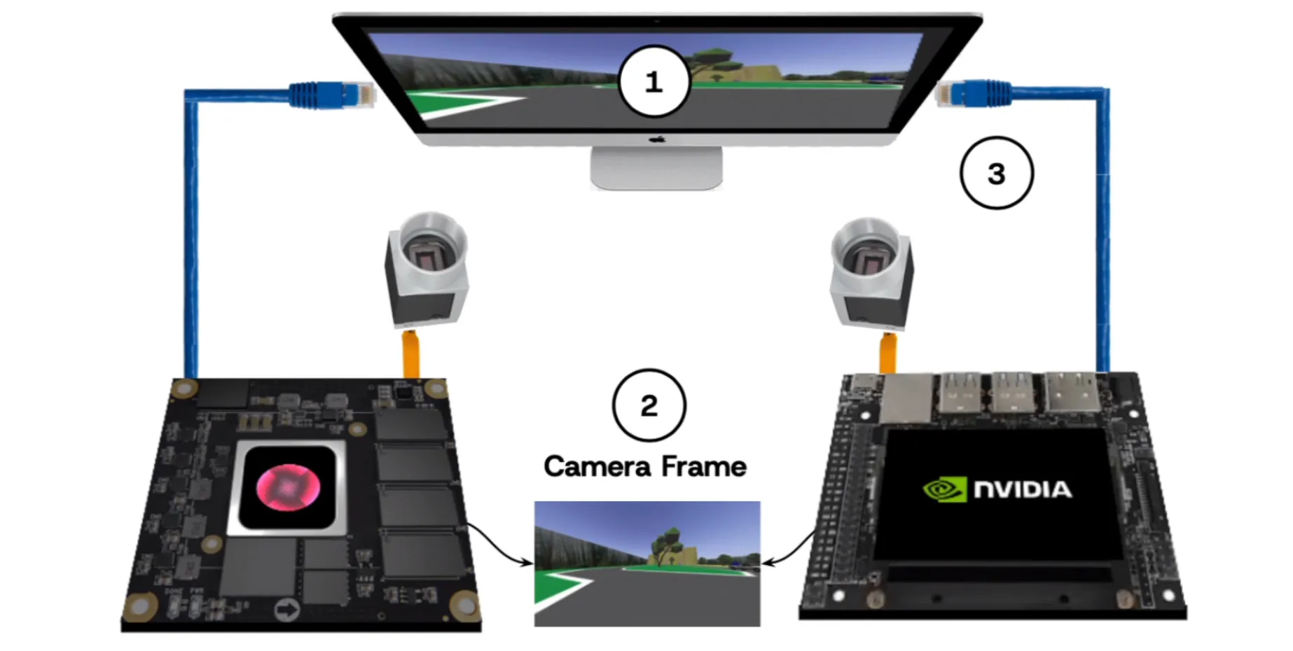
We have a simulated self-driving system where both computers compete to drive around a course as quickly and safely (not crashing into obstacles) as possible. The data flow for each computer is:

1. Capturing the simulated dashcam view on a monitor (camera I/O);
2. Run a CNN model on the camera feed to get driving decisions;
3. Send decisions back to simulation controller through a USB connection.

ML architecture

As you’ll come to see, the abstraction of an ML model as a graph of mathematical operations will be useful later on. We used ONNX (Open Neural Network eXchange) to save our models as graphs, the final one shown below:

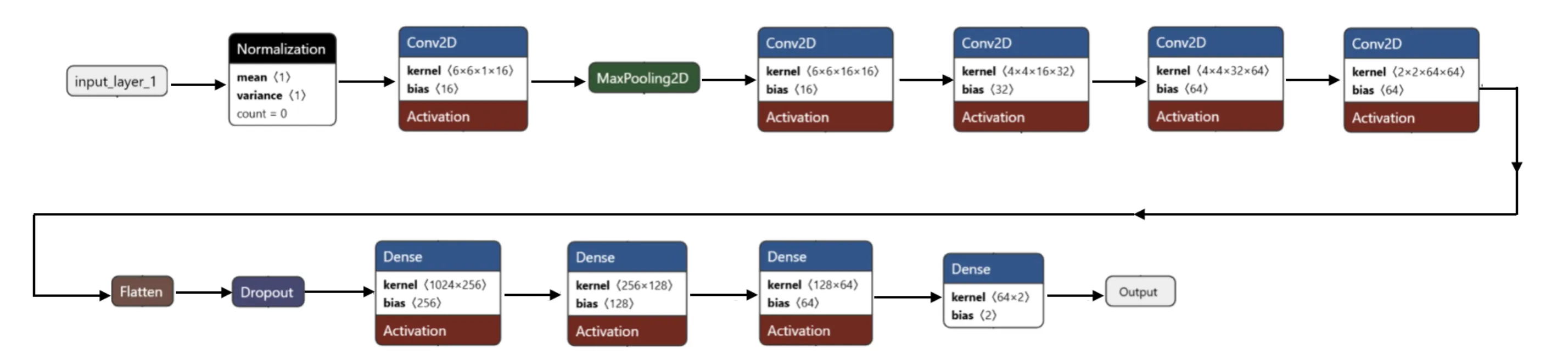
The main thing I want you to take away from the graph is that we’re doing convolution layers and dense layers. Additionally, the CNN was trained using imitation learning. To put it simply, one of us manually drove around the simulated track to create a training dataset of dash cam images and the associated moves, and we trained on that.

Neuromorphic Compute

IBM Northpole

I’ve already talked quite a bit about IBM’s NorthPole, so I’ll keep this part quick. The NorthPole architecture is a “distributed, modular core array (16x16), with each core capable of massive parallelism (8192 2-bit operations per cycle)”. All these cores come equipped with their own memory, essentially keeping all resource usage “localized” and thus speedy. Here’s a comparison between a GPU memory layout, Google’s TPU and the NorthPole’s:

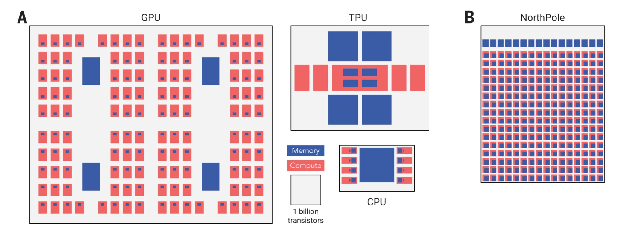
The cores are interconnected by a high-speed, high-throughput network-on-chip (NoC, and actually it’s a few of them).

AMD Versal

Given the constraints of the project, we couldn’t design, route and manufacture a unique chip. Thankfully, AMD had already released the first generation of its Versal line. The Versal is a System-on-Chip (SoC). This means the silicon is split into two “domains”: The “soft” silicon, the configurable FPGA part, and the “hard” silicon, constrained and fixed ICs. The latter is usually a few CPUs, but the Versal comes with the AI Engine Array as well:

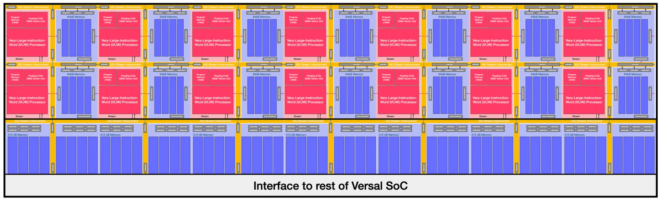
This should look familiar: a row of memory (blue) followed by a homogeneous grid of interconnected parallel processors (red & blue). It is precisely the neuromorphic model of compute presented in the NorthPole paper.

Each processor can access its own 64kB local memory buffer and the ones adjacent to it. The memory array at the bottom is composed of many 512kB shared buffers that can be accessed by several compute tiles at once. All the tiles are linked by the AXI-Stream Interconnect, which works similarly as the NoC in the NorthPole.

Implementation

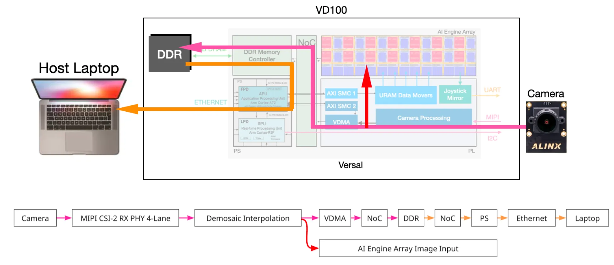
We got the Versal on a very well priced board from Alinx, the VD100 with the following peripherals (specifically we got the xvce2302-sfva784-1lP-e-S version):

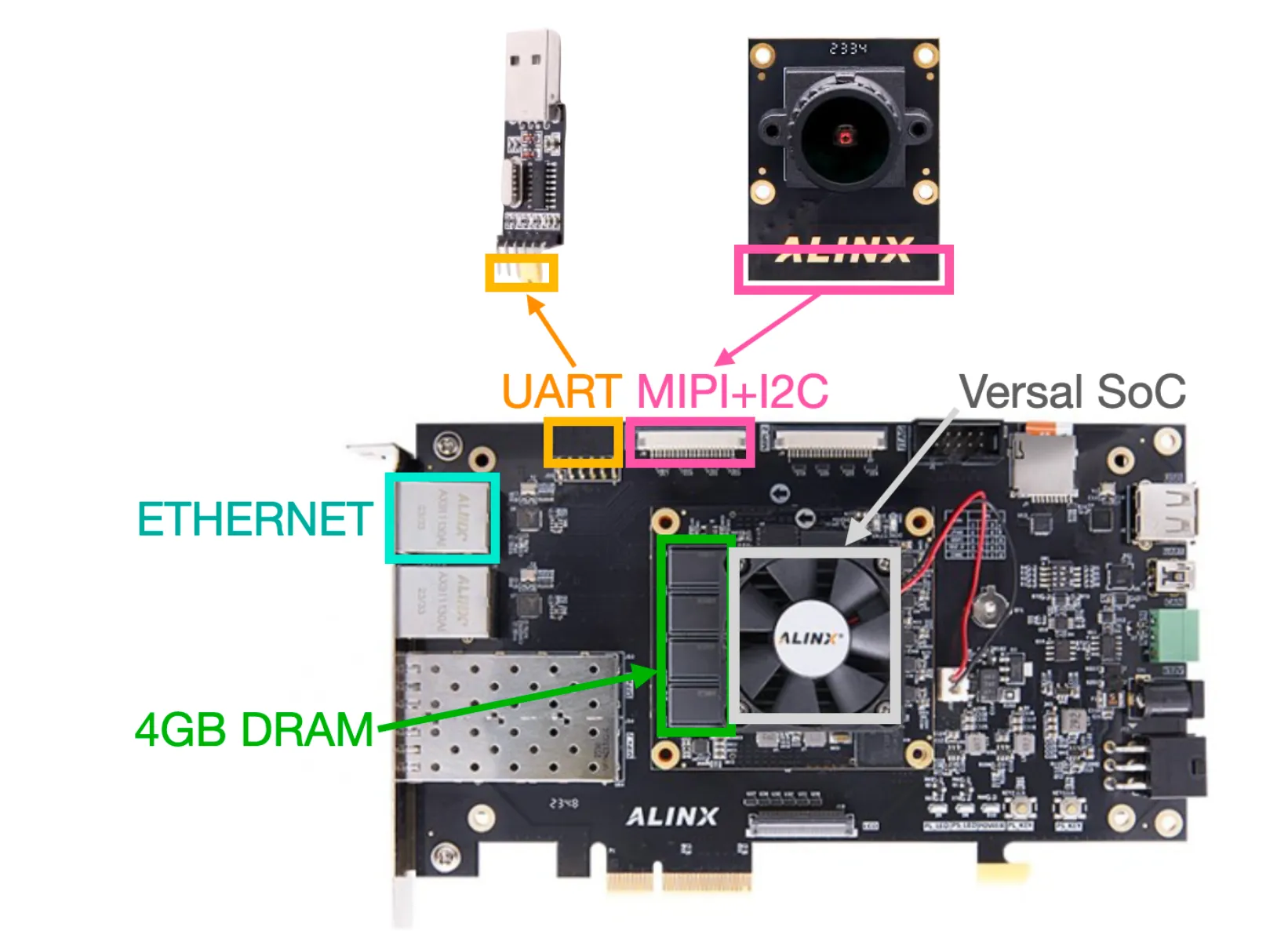
We’ll use the MIPI to connect with high-bandwidth cameras serving as the “eyes” to the self-driving model. The I2C port is also used to initialize camera settings like resolution, AWB, gain. The Ethernet port was used for communicating images between the board and our laptops (to check training data) and UART is used for sending driving decisions back to the simulator.

The micro-architecture we’ll need then should look something like this:

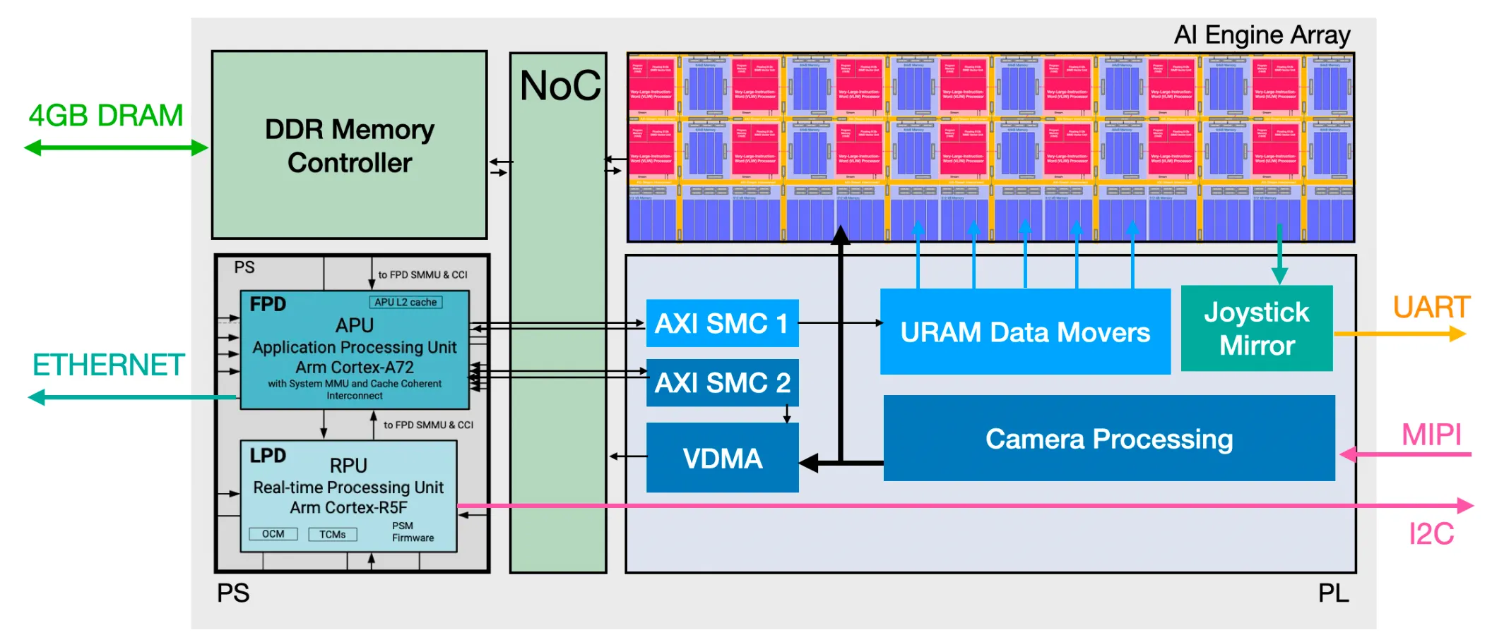
There are four partitions here:

• AI Engine Array: That’s the neuromorphic compute grid that the neural network (inference) will run on.
• Programmable Logic (PL): The reconfigurable FPGA partition of the Versal; we’ll use it to decode the MIPI data stream and feed it into the AI Engine array.
• Programmable System (PS): This is a small group of ARM processors to boot the system, initialize the AI Engines, cameras and ethernet.
• NoC: Connects the PS, PL and AIE Array together, as well as the off-chip 4GB DRAM.

Now for some practical details. This is the exact CNN we are going to run:

Note that the last layer has two dimensions, left or right for the car. To keep it simple we let it drive at constant speed.

I won’t go too much into detail on the kernel design because that’s what the last post was about. Read it for more context, I’ll just give a brief explanation of how each layer (type) went.

Kernels and parallelism

The input layer is the 580x196x1 image, stored in a Memory Tile (because it’s big). We combined the convolution operation with the max-pooling, so we take an 8x8 patch of the input image, convolve on four 6x6 regions, each giving 1x1x16 features, then perform max-pool on those four.

There are four of these kernels handling a quadrant of the image in parallel (something you’ll see we do everywhere). The following convolutions don’t do any max-pooling, which makes it much easier. The further shapes are not quite as big, so we process them in two vertical chunks instead.

The dense layers is not much different from the input convolution layer, instead of an image with pixel density filters applied (convolution), it’s a big matrix with partial products applied. It still makes sense to split it into sections and distribute the compute.

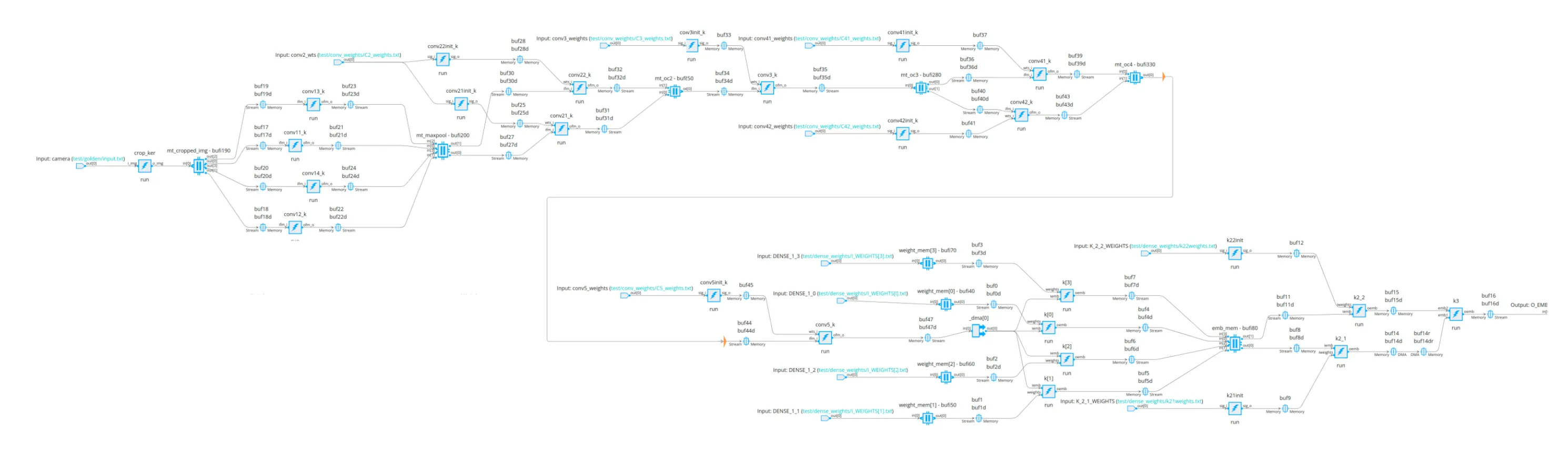
I don’t know how legible this is, but it’s the full compute graph for the CNN. This dictates the flow of data to perform inference:

This graph representation itself is not sufficient to run in actual hardware, of course. The last step is to assign each kernel a Compute Tile (a physical memory location in the grid) and the same for the Memory Tiles:

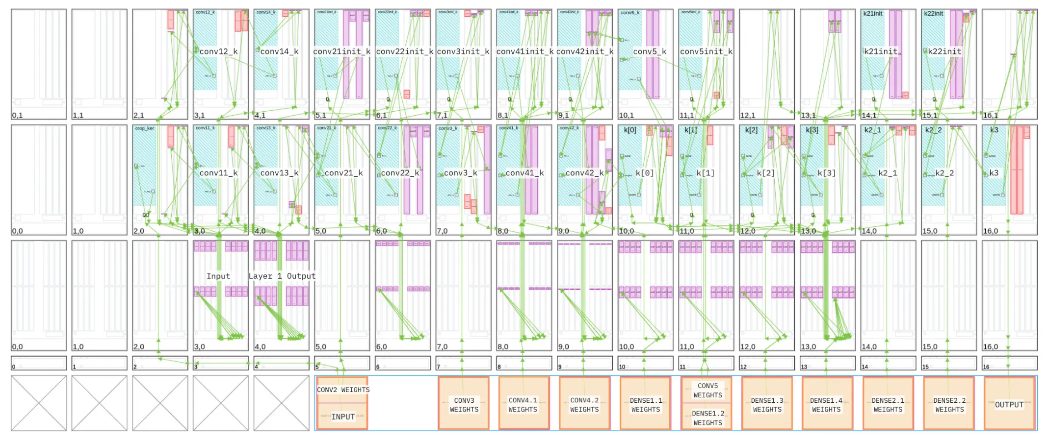
Cyan represents the active Compute Tiles, purple the memory regions (64kB data memory or a dedicated tile) and green arrows are physical connections from kernel to kernel.

In the bottom, the orange regions shows external connections to the rest of the chip. That is, the input camera feed and the output to the car controller. We also used an AMD Kernel called weights_init to load the weights through a stream from the PL. From these external connections, I want you to notice that once data enters the AIE Array, it only leaves once all computation is done (the output). This is exactly the “brain-like” compute we want.

Camera connectivity

With the compute established, we now need to get the data from the camera (MIPI) feed. This was implemented in the PL region as follows:

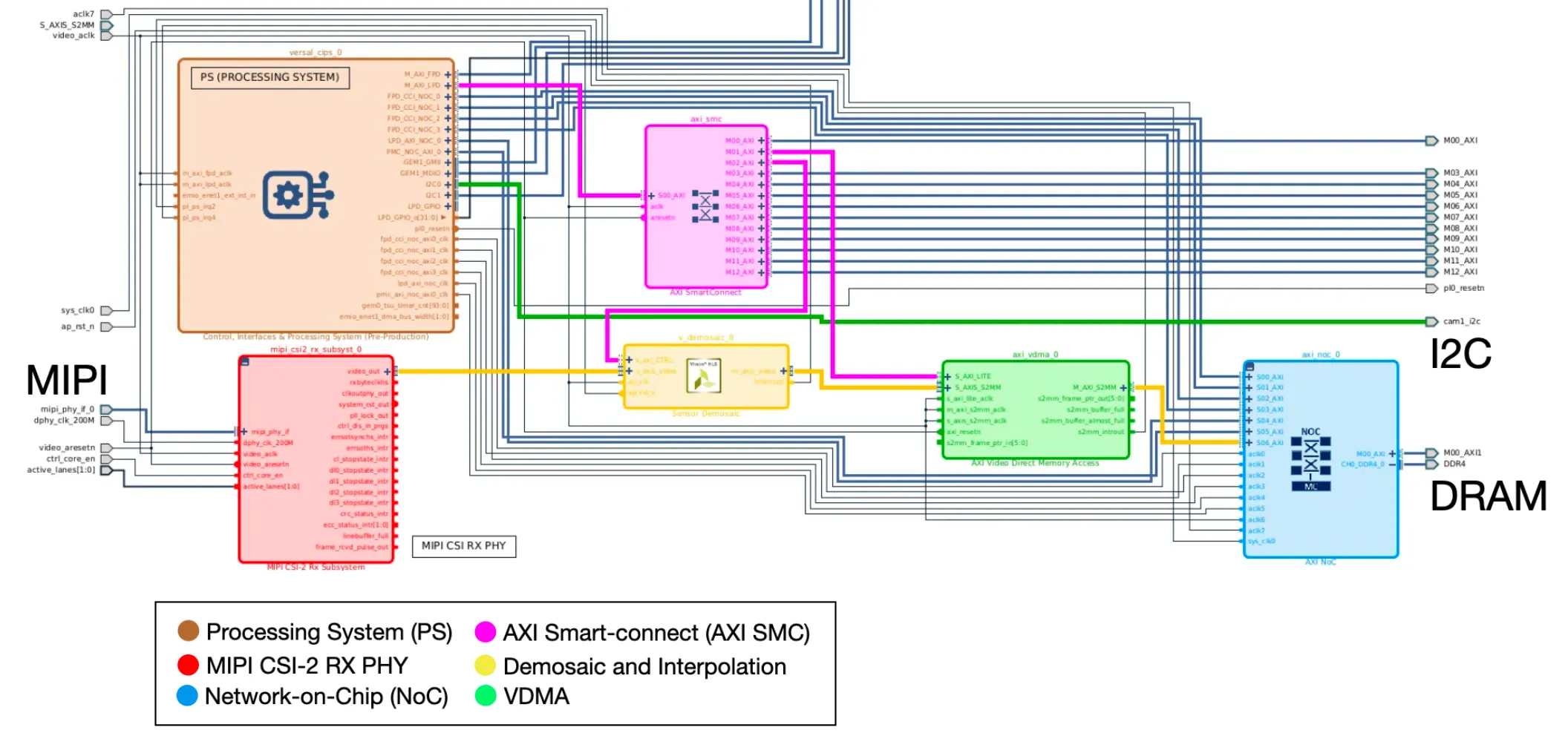
The green wire extending from the PS (big orange block) is the direct I2C connection to the camera. We use this to initialize the camera capture settings.

The PS then communicates to the “Demosaic and VDMA blocks” through AXI Smart-Connect (SMC). Then we can set more useful variables like video image size and pixel resolution through some C++ firmware.

The camera we used (Alinx AN5020) uses the industry-standard MIPI CSI-2 (Camera Serial Interface) protocol. Physically, we implemented MIPI 4-lane, where 10 signal lines (8 data, 2 clock) enter the chip. These signals go into a MIPI CSI-2 receiver-physical (RX PHY) layer that synchronizes and writes the data to an AXI-Stream interface. That’s a lot of buzzwords, but very important, because it’s how we get a crucial advantage over the Jetson, which obtains data via MIPI 2-lane, half the bandwith of our interface. That’s the benefit of having reconfigurable hardware, not too shabby.

Brief aside: demosaicing. The raw data values received by the RX PHY are not full-color, but rather a mosaic of brightness (scalar) values filtered through something called a Bayer pattern, where each pixel only gets one color (red, green, or blue). It looks something like this:

Because green contributes more to perceived sharpness in human vision, it is sampled twice as often as red or blue.

To convert this into single-channel, full-clor RGB, we need to apply the demosaicing algorithm, which estimates the missing color components at each pixel using surrounding information. For example, to get the green value at a red pixel $(i,j)$ we use bilinear interpolation of the vertical and horizontal neighbors:

Similarly, red at green uses the diagonal neighbors. There are fancier methods based on frequency but this is great fast option for our application.

Coming out from the demosaic block is the final AXI-Stream of 8-bit RGB data representing the full color image seen by the camera. The broadcast happens in two directions — one directly to the input port of the compute grid for inference, and another to VDMA.

Video Direct Memory Access (VDMA)

As the name suggests, the VDMA takes in the video stream from the Demosaic, formats it as a memory-mapped transaction, and writes the data through the NoC to the DDR4 that resides off-chip. This enables the PS to read the camera frame from DDR4 itself, and send the image over Ethernet to a host computer on the same local network. With this, we can inspect the video feed, focus the camera lens, and collect training samples for our self-driving model.

The PS runs a TCP server, using the lwip TCP/IP stack library. Any client on the same local network as the board can connect using Python’s simple socket library. In the PS firmware, we register a custom callback function tcp_recv_callback that will run every time an external client sends a 256 bytes packet to the board. The first 8 bytes of this packet tell tcp_recv_callback what data to send back – this could be a camera frame, a value of a register, or an output of the AI Engine. The maximum return packet size is 32768 bytes.

The board uses a JL2121 Ethernet PHY to convert TCP actions into electrical signals over Ethernet. This is not a chip natively supported by lwip so we had to make a custom build for our case.

Sending model predictions to sim

After we run inference and obtain the output, the data is written out to the VD100’s UART port. These signals go to a USB-TTL device plugged into the simulation laptop, so that from the perspective of the simulator, a controller is making the moves. The UART uses 8 data bits, 1 stop bit, and 0 parity bits.

Finally the systems full flow of data looks something like this:

Testing and results

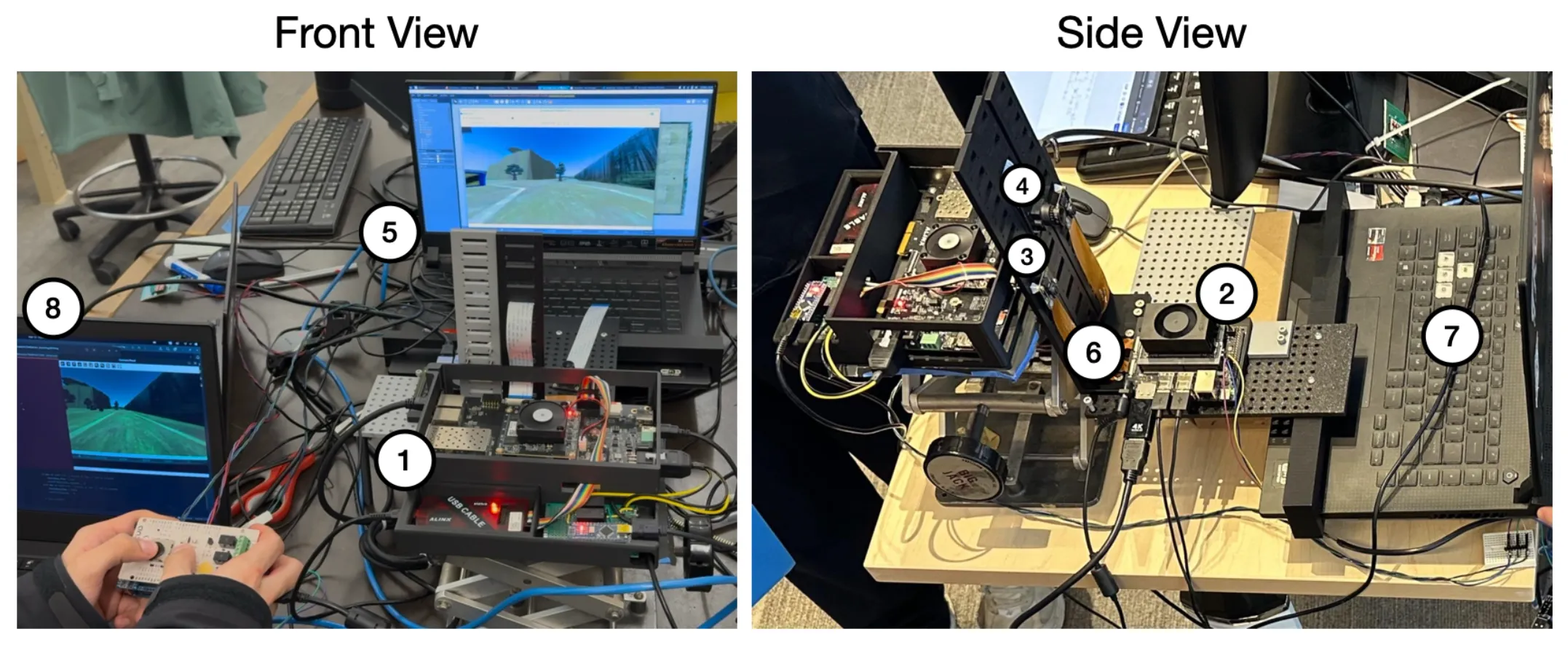
Below is our somewhat clunky testing setup, with the components:

1. 1×IRIX enclosure with:
   • Alinx VD100
   • Digilent JTAG Programmer (red)
   • Arduino Power Manager
2. 1×NVIDIA Jetson Orin Nano 8GB
3. 1×Raspberry Pi Camera V2.2 with cable
4. 1×Alinx AN5020 MIPI Camera with cable
5. 1×3-way Ethernet Switch, 3×Ethernet cables
6. 1×G17 Laptop camera mount
7. Computer with Ethernet and multiple USB ports to upload programs, turn the board on, read serial statements, and obtain camera frames.
8. ROG Strix G17, the laptop running the simulation.

We measured the following figures:

Note that we did not run a TensorRT model on the Jetson, mostly because the update gave us some trouble on other firmware drivers we needed, although some isolated experiments still seem to give us the edge.

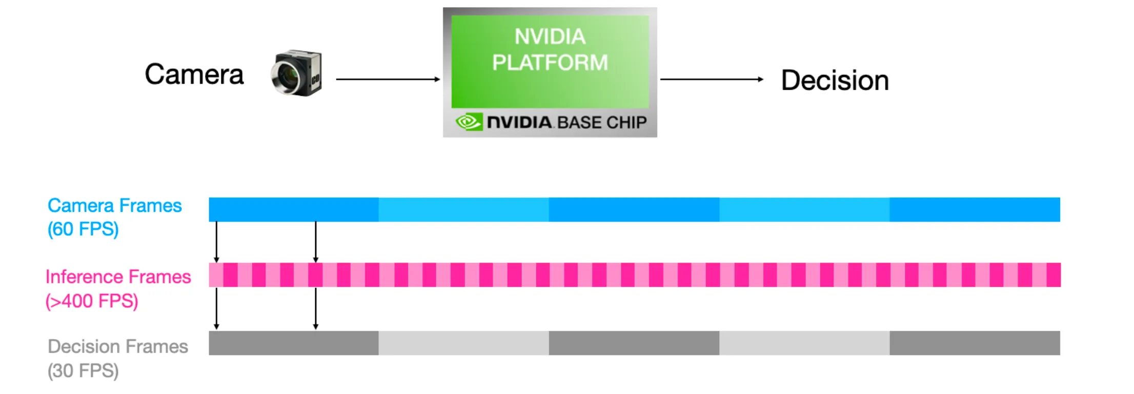
Qualitatively, our architecture runs the model much better than the Jetson. In terms of driving, we observe that the driving agent in the simulator is capable of following the track more con- perform quick turns that the Jetson consistently fails at. This is not due to the model’s performance as we have probed the track for output predictions which match correct actions.

We think this is due to input frame-rate bottleneck on the Jetson, where it runs inference multiple times on the same camera frame:

Takeaways and stuff

There are still some limitations. Our project only supports camera inputs and CNN models. Deploying a general-purpose Edge AI solution would require more sensors and more kernels (to be written). Ideally, we could have a model compiler that takes ONNX files and maps them to adequate AI Engine graphs (pulling from some library of kernels and methods, maybe). It would also handle quantization, buffer assignment and data flow. This is not so far removed from CUDA itself, which has largely helped NVIDIA’s hardware to flourish.

Overall, I’m pretty happy with how it turned out, especially that we managed to get some sort of edge over an NVIDIA product. I expect Edge AI to become a massive area of focus in the coming years, probably already starting now.

See you all next time.